How to Generate a Transfer Function Using HARKTOOL5
Table of Contents
1. Introduction
2. Measurement-based Transfer Function Generation
3. Geometric-calculation-based Transfer Function Generation
4. Evaluating Transfer Functions
1. Introduction
A transfer function in HARK is defined as a complex spectral function to represent the relationship in wave propagation between a microphone array and a sound source. HARK uses two types of transfer function data sets; one is to localize sound sources(sound source localization), which is called localization transfer function. The other is to separate a mixture of multiple sound sources (sound source separation), which is called separation transfer function.
1.1. Sound Source Localization
In HARK, sound source localization is estimating the direction of the sound source in 1 or 2 dimensions. For 1D localization, HARK can estimate the angle between a reference direction and sound source direction on a horizontal surface or the azimuth (Figure 1). For 2D localization, HARK can be extended so that once the azimuth has been estimated, HARK will also estimate the angle between the horizontal surface and the vertical position of the sound source or the elevation (Figure 2). The location of multiple sound source can be estimated at the same time for both 1D (Figure 3) and 2D (Figure 4).
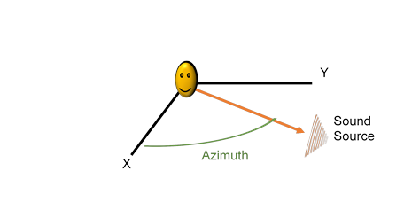
Figure 1. Example of locating of a single sound source in 1D in HARK
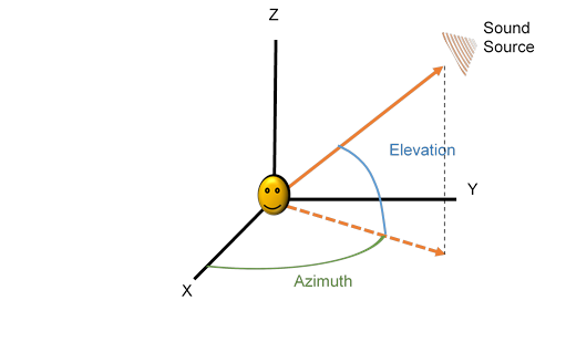
Figure 2. Example of locating of a single sound source in 2D in HARK
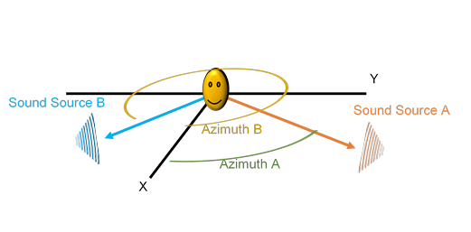
Figure 3. Example of locating of multiple simultaneous sound sources in 1D in HARK
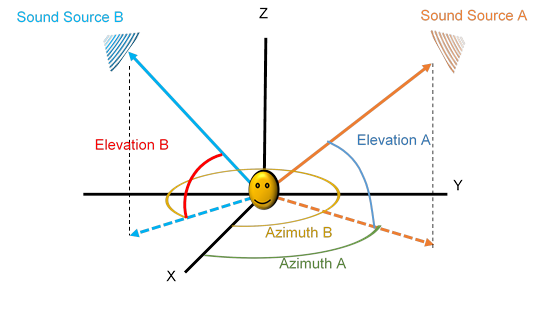
Figure 4. Example of locating of multiple simultaneous sound sources in 2D in HARK
LocalizeMUSIC is one of HARK's main nodes used for Sound Source Localization. This node provides MUltiple SIgnal Classification (MUSIC) methods to estimate sound source directions with its individual spectral power. A MUSIC method uses a set of transfer functions where each transfer function represents sound propagation from a sound source to a microphone array. LocalizeMUSIC compares the input signal with each transfer function contained in the set, then it will select the best matching transfer function based on the input signal's propagation characteristics and that of the transfer functions. The best matched propagation characteristics will indicate the general direction of the sound source.
For more information on LocalizeMUSIC and the MUSIC algorithm, please refer to the HARK Document at https://hark.jp/document/document-en/.
1.2. Sound Source Separation
Hark can separate inputted sound mixtures into a set of separated sounds. This is called sound source separation. Figure 5 shows an overview of sound source separation. The algorithms to perform sound source separation require location information of sound sources as an input. The location information on sound sources can be obtained directly from sound source localization, or the information can be set with constant values. Sound source separation also uses a set of transfer functions to estimate a separation matrix which is necessary for a separation process.
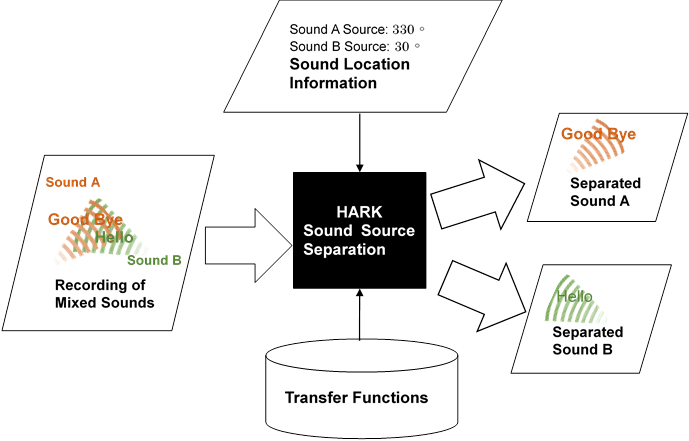
Figure 5. A sound mixture is separated into the separated sounds using the sound location information and transfer functions
GHDSS and BeamForming can be used for sound source separation. For more information, please refer to the HARK Document at https://hark.jp/document/document-en/.
1.3. Methods to generate transfer functions
If we wish to record a sound originating from a sound source, it is important to understand that the recorded sound data will not exactly match that of the originating sound source due to reflected sounds better known as reverberation. For instance, as shown in Figure 6, let's consider that we have a loudspeaker, a microphone array, and an object positioned in a room surrounded by four walls. When a sound signal is emitted from the loudspeaker, the emitted sound signal is reflected by the walls and/or the object before arriving at the microphone array (Reflected Sound). This will cause delays and changes to the recorded sound data recorded by the microphone array.
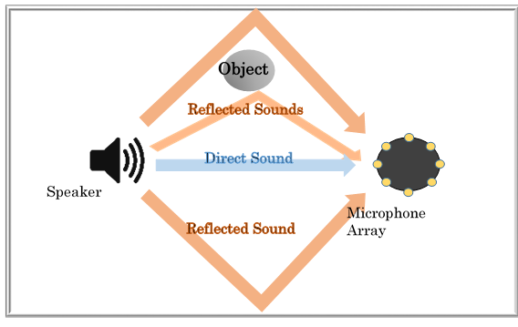
Figure 6. Sound traveling from a speaker to a microphone array in a room with four walls and an object. [Top View]
The characteristics of this propagation is represented in the transfer functions. The transfer functions can be obtained by actual measurements or numerical simulation with the geometric relationship between a microphone array and sound sources.
1.3.1. Measurement-based method
This method uses recorded TSP (Time Stretched Pulse) responses, or impulse responses to generate the transfer functions.
An impulse response is the signal recorded by a microphone array for an impulse signal emitted from a sound source. The impulse signal contains signals at all frequencies in a single point in time. The problem in measuring the impulse response is that a large amount of power is necessary for emitting a maintainable high signal-to-noise ratio (SNR) sound, which is difficult to achieve using a conventional loudspeaker.
To solve this problem, a Time Stretched Pulse (TSP) signal is alternatively used. The TSP signal is obtained by stretching out the frequencies of the impulse signal over time. Figure 7 shows spectrograms of the impulse and TSP signal. For the impulse signal, all the frequencies are concentrated within an instantaneous period, and for the TSP signal, the frequencies are stretched over time.
Stretching out the frequency allows each frequency to be played at maximum power. The signal can be repeated multiple times which improves SNR of the recorded TSP signal by averaging. The impulse response can be calculated from the TSP response.
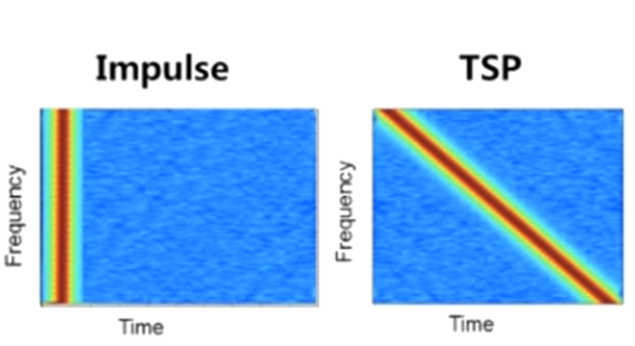
Figure 7. A graph of the spectrum of frequencies of the Impulse and Time Stretched Pulse (TSP) signal over time.
1.3.2. Geometric-calculation-based method
This method uses listed location data of both sound sources and microphones to generate the transfer functions.
Impulse responses are simulated from the microphone positions and sound source positions. From these impulse responses, the transfer functions are generated on the assumption that the microphones are set in a free space. This assumes that sound reflections from the object in Figure 6 are ignored. For this reason, transfer functions generated using this method are less accurate than those generated using the measurement-based method.
2. Measurement-based Transfer Function Generation
This section will discuss how to generate transfer functions from actual measurements using TSP. This can be divided to two parts: (1) playing and recording the TSP signal, and (2) calculating impulse responses from TSP responses. The steps for recording TSP signals differ for each type of recording device, and they are covered in extra manuals.
The impulse response for each recorded TSP response can be calculated from the TSP response. This calculation can be performed using HARTOOL (see Figure 8). HARTOOL creates transfer functions from the calculated impulse responses.
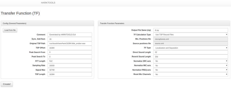
Figure 8. Calculating the transfer function using HARTOOL5
To generate measurement-based transfer functions, recording TSP responses is essential. TSP responses can be obtained in two different ways; synchronized recording and unsynchronized recording. Synchronized recording requires special equipment (e.g., RASP series), but it provides accurate transfer functions which gives the best performance in sound source localization and separation. On the other hand, unsynchronized recording can be done with most microphone array devices, but it may provide poor performance in sound source localization and separation compared to synchronous recording because it provides less accurate transfer functions.
The transfer functions will perform best when the TSP responses are recorded in the same set-up where the transfer functions are to be used. However, it can happen that it is difficult to record TSP responses in the same set-up. The recording set-up needs a loudspeaker to play the TSP signals and a microphone array to record the responses. The position of both the loudspeaker and the microphone array for every recording needs to be precise. The TSP signal needs to be played multiple times in order to reduce the impact of background noise and reverberation when creating the transfer function. The TSP signal must be played from all directions where sound source localization and or sound source separation are to be performed by the transfer functions generated using the TSP responses. The recording setup's environment can affect the difficulty of performing this procedure. For example, if the recording setup is located in a public place such as a park, then conducting this procedures can be difficult. When the recording cannot be done in the same set-up where the transfer function is to be used, please find a more suitable environment. To make a transfer function which works in most environments, please record TSP responses by moving a loudspeaker in a circle at the 5° intervals in a noise free environment. The obtained transfer functions are less accurate than those generated in the same set-up, however, they are generally more accurate than the transfer function created using Geometric-calculation-based method. Please note that the accuracy of transfer functions may not be directly related to localization and separation performance.
Figure 9 shows a sample set-up of how a TSP response is recorded from every direction with 30° intervals (recommended interval is 5°). The recording environment is assumed to be noise free and without presence of any object. A microphone array is placed at the center of a circle with a radius of 1 m. Decide a starting point where you will begin recording and mark it as 0°. Then, mark the rest of the positions of the loudspeaker every 30° interval on the circle's circumference. When starting the recording, place the speaker on the starting point marked as 0°. After successfully obtaining the data by playing the TSP signal multiple times, move the speaker to the next position as shown in Figure 9. For the recording set-up with 30° intervals indicated in Figure 9, the recording needs to be done at 12 different positions.
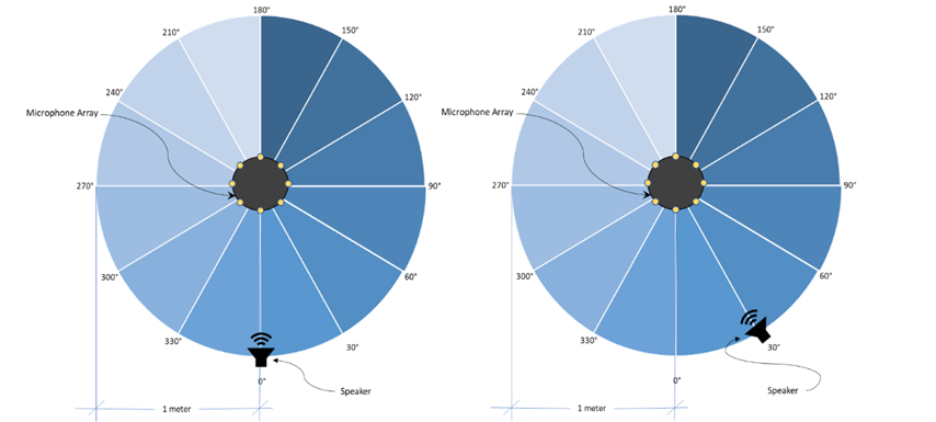
Figure 9. Speaker Positions [Top View]
Please note that the direction of the TSP signal recorded is significant to determine the capability of the transfer functions. For example, the direction of a sound source played at 130° cannot be detected precisely when the transfer function was generated using TSP responses with 30° interval in a circular set-up. HARK will output the direction information 120° (Figure 10).
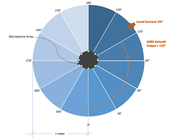
Figure 10. Sound source localization for a set-up with a sound source at 130° but using a transfer function generated using impulse response with 30° interval [Top View]
When the recording can be done in the same set-up, please refer to Figure 11 which will demonstrate an example setup. Figure 11 shows a bar setup environment, and a bartender is standing behind a bar counter. Customers are giving orders to the bartender across the bar counter. In this example setup, we have replaced the bartender with a robot equipped with hark. It is best to record TSP responses in the same recording environment in order to get the best performance. The sample set-up illustrates how to record TSP responses for the transfer functions to perform both sound source localization and sound source separation of simultaneous orders in a bar.
Suppose there are up to 5 customers who wish to place an order as shown in Figure 11 (a). Assuming that the positions of customers surrounding the bartender are all in the same intervals, say, 30°, shown in Figure 11 (b). Then, place a microphone array in the bartender position as shown in Figure 11 (b) and place a loudspeaker in the 1st customer's position. The height of the microphone array and the speaker must be the same, although in real situations the height may vary. Record the TSP responses and then move the speaker to the next customer position. Repeat this for all 5 positions. The transfer functions generated using TSP responses recorded in the Figure 11 (b) setting will perform best on localizing and separating sound sources in the Figure 11 (a) setting.
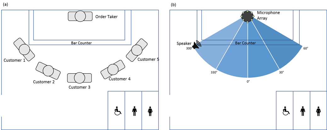
Figure 11. Bar set-up [Top View], (a) an order taker and the customers, facing each other across the bar counter,
(b) a microphone array and a speaker are being placed in the positions of the order taker and the customer respectively.
2.1.1. Recording Equipment
Recording equipment (microphone array, recording tool, etc.) and the settings (source position, etc.) should be carefully chosen depending on the purpose. Three different recording procedures are provided. The sample conditions of recording set-ups used in these recording procedures are described in Table 1.
Table 1. TSP Recording set-up condition example
| Microphone array | Recording Tool | Synchronized/Unsynchronized | SRC Position | ||
| Type | Radius | Interval | |||
| TAMAGO-02 | HARK-Designer | Unsynchronized | Circular: 0°-360° | 1m | 30° |
| RASP-ZX + Mic | HARK-Designer | Synchronized | Circular: 0°-360° | 1m | 30° |
| RASP-24 + Mic | Wios | Synchronized | Circular: 0°-180° | 1.2m | 30° |
Figure 12 shows TAMAGO described in the first row of Table 1.
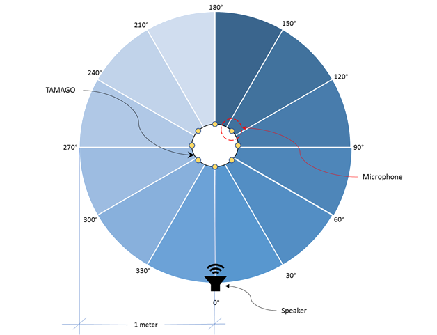
Figure 12. TAMAGO Recording Environment Set Up [Top View]
2.1.2. Recording Tool
Any recording tool can be used.
We recommend using one of the following tools which has a function of multi-channel recording:
- HARK-Designer
- Wios
2.1.3. Recording the TSP signal procedure examples
The procedure for recording TSP Response will be slightly different depending on the equipment. The detailed procedure for the following HARK supported hardware are provided as separate manuals.
- Recording TSP Response using TAMAGO
- Recording TSP Response using RASP-ZX
- Recording TSP Response using RASP-24
2.2. Transfer Function Generation
After recording the TSP responses, the transfer functions can be generated from the TSP response wav files with HARKTOOL5. In addition, the Microphone Array Position XML and Sound Source Position XML are necessary as shown in the Figure 13.
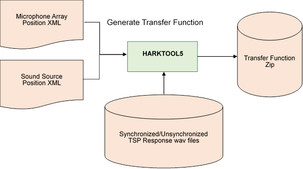
Figure 13. Transfer function generation by Measurement-based method
2.2.1. HARKTOOL List File
The template files for both microphone array positions and sound source positions are generated by HARKTOOL5. For a Spherical or Cylindrical layout, HARKTOOL5 auto-generates template files with the positions of the microphones and sound sources. To specify another layout, the xml file needs to be edited manually. The Table 2 highlights the requirements for the contents of setting file in the measurement-based method.
Table 2. HARKTOOL list files requirements for Measurement-based method
| Method | Microphone Array Positions XML | Sound Source Positions XML |
| Measurement-based Method | The number of microphones should be correctly specified. The attribute for x, y and z positions needs to be filled with any non-null number string. | The positions where the loudspeaker played the TSP signal should be specified as accurate as possible. The path of a wav file for recorded TSP responses should be correctly specified. |
2.2.1.1. Array Positions XML
The file for Microphone Array Positions XML should contain the number of microphones and the location information on all microphones. Table 3 shows a sample Microphone Array Positions XML for Measurement-based method. The number of position element must match the number of microphones in the microphone array. The x, y and z attributes of each position element can be set to any non-null number string (highlighted in blue).Table 3. Sample Microphone Array Positions XML for Measurement-based method.
|
<hark_xml version="1.3"> <positions type="microphone" frame="0" coordinate="cartesian"> <position x="0.0365" y="0.0000" z="0.0000" id="0" path=""/> <position x="0.0258" y="0.0258" z="0.0000" id="1" path=""/> <position x="0.0000" y="0.0365" z="0.0000" id="2" path=""/> <position x="-0.0258" y="0.0258" z="0.0000" id="3" path=""/> <position x="-0.0365" y="0.0000" z="0.0000" id="4" path=""/> <position x="-0.0258" y="-0.0258" z="0.0000" id="5" path=""/> <position x="0.0000" y="-0.0365" z="0.0000" id="6" path=""/> <position x="0.0258" y="-0.0258" z="0.0000" id="7" path=""/> </positions> </hark_xml> |
2.2.1.2. Sound Source Positions XML
The file for Sound Source Positions XML contains both sound source positions and TSP response filenames. Table 4 shows a sample Sound Source Positions XML for Measurement-based method. The x, y and z attributes in each position element describe each position where a loudspeaker played the TSP signal (highlighted in blue). The path attribute in each position element specifies a TSP responses wav file path (highlighted in red).Table 4. Sample Sound Source Positions XML for Measurement-based method.
|
<hark_xml version="1.3"> <positions type="TSP" coordinate="cartesian"> <position x="1.0000" y="0.0000" z="0.0000" id="0" path="/home/user/tamago_rec/sep_0_0.wav"/> <position x="0.8660" y="0.5000" z="0.0000" id="1" path="/home/user/tamago_rec/sep_0_30.wav"/> <position x="0.5000" y="0.8660" z="0.0000" id="2" path="/home/user/tamago_rec/sep_0_60.wav"/> <position x="0.0000" y="1.0000" z="0.0000" id="3" path="/home/user/tamago_rec/sep_0_90.wav"/> <position x="-0.5000" y="0.8660" z="0.0000" id="4" path="/home/user/tamago_rec/sep_0_120.wav"/> <position x="-0.8660" y="0.5000" z="0.0000" id="5" path="/home/user/tamago_rec/sep_0_150.wav"/> <position x="-1.0000" y="0.0000" z="0.0000" id="6" path="/home/user/tamago_rec/sep_0_180.wav"/> <position x="-0.8660" y="-0.5000" z="0.0000" id="7" path="/home/user/tamago_rec/sep_0_210.wav"/> <position x="-0.5000" y="-0.8660" z="0.0000" id="8" path="/home/user/tamago_rec/sep_0_240.wav"/> <position x="0.0000" y="-1.0000" z="0.0000" id="9" path="/home/user/tamago_rec/sep_0_270.wav"/> <position x="0.5000" y="-0.8660" z="0.0000" id="10" path="/home/user/tamago_rec/sep_0_300.wav"/> <position x="0.8660" y="-0.5000" z="0.0000" id="11" path="/home/user/tamago_rec/sep_0_330.wav"/> </positions> <neighbors algorithm="NearestNeighbor"> <neighbor id="0" ids="0;"/> <neighbor id="1" ids="1;"/> <neighbor id="2" ids="2;"/> <neighbor id="3" ids="3;"/> <neighbor id="4" ids="4;"/> <neighbor id="5" ids="5;"/> <neighbor id="6" ids="6;"/> <neighbor id="7" ids="7;"/> <neighbor id="8" ids="8;"/> <neighbor id="9" ids="9;"/> <neighbor id="10" ids="10;"/> <neighbor id="11" ids="11;"/> </neighbors/> </hark_xml> |
2.2.2. Generating Transfer Function Examples
HARKTOOL5 is used to generate the transfer functions based on the Microphone Array Positions XML, Sound Source Positions XML, and the TSP Response recording wav files. Transfer function generation procedures by Measurement-based method using the following HARK supported hardware are provided as separate manuals.
- Generating a Measurement-based Transfer Function for TAMAGO Using HARKTOOL5
- Generating a Measurement-based Transfer Function for RASP-ZX Using HARKTOOL5 (available soon)
A video version of the steps can be found in https://www.youtube.com/watch?v=vvrbaTa7Nek.
3. Geometric-calculation-based Transfer Function Generation
This section will discuss generating transfer functions using the Geometric-calculation-based method. In this method, impulse responses will be obtained by numerical calculation with the geometric relationship between microphones and sound sources rather than by the actual measurement of the response which is required in Measurement-based method (see Section 2.1 Recording TSP response).
Geometric calculation-based method assumes that both the sound source and microphones are placed in a free space. "Free space" means there are no obstructive objects, walls and floor in the space which would cause sound reflecting off the environment, so the sound would travel without any changes from the original sound source. Figure 14 illustrates the difference in how sound travels from a speaker to a microphone array in a limited space and in a free space. Figure 14 (a) shows both "Direct sound", sound not affected by the environment, and "Reflected sound," sound reflecting off the environment, which normally happens in the real world. Figure 14 (b) shows only "Direct sound" traveling in an infinitely large space without walls or objects.
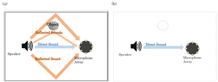
Figure 14. (a) Sound traveling from a speaker to a microphone array placed in a room with four walls and an object. (b) Sound traveling from a speaker to a microphone array in free space. [Top View]
Since Geometric-calculation-based method does not take into account the effects on sound due to the environment by excluding reflected sound when generating transfer function, the performance of the transfer functions generated using this method will be generally lower than the ones generated using the Measurement-based method. The user will have to evaluate if the transfer function generated by this method will provide the desired performance level.
3.1. Transfer Function Generation
In this method, transfer functions can be generated without using any pre-recorded TSP response data required for Measurement-based method. Instead, impulse response will be simulated using microphone position information and sound source position information (Figure 15).
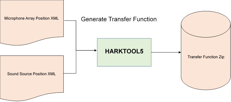
Figure 15. Geometric-calculation-based Transfer Function Generation
3.1.1. HARKTOOL list file
The template files for both microphone array positions and sound source positions are generated by HARKTOOL5 For a Spherical or Cylindrical layout, HARKTOOL5 auto-generates template files with the positions of the microphones and sound sources. To specify another layout, the xml file needs to be edited manually. The Table 5 highlights the requirements for the contents of setting file in the geometric-calculation-based method.
Table 5. HARKTOOL list files requirements for Geometric-calculation-based method
| Method | Microphone Array Positions XML | Sound Source Positions XML |
| Geometric-calculation-based Method | Both the number of microphones and the position for each microphone should be correctly specified. | The sound source positions to simulate the impulse response should be specified as accurate as possible. The attribute for file path needs to be filled with any non-null string. |
3.1.1.1. Array Positions XML
The file for Microphone Array Positions XML should contain the number of microphones and the location information on all microphones. For transfer function generation using geometric-calculation-based method, the file for microphone array positions XML must contain the correct number of positions element. The number of position element must match the number of microphones in the microphone array. The x, y and z attributes of each position element should accurately describe the position of each microphone in the microphone array. The location information on all microphones will be used to simulate the impulse responses. Table 6 shows a sample Microphone Array Positions XML for Geometric-calculation-based method. The x, y and z attributes in each position element describe the position of each microphone in the microphone array (highlighted in blue).Table 6. Sample Microphone Array Positions XML for Geometric-calculation-based method.
|
<hark_xml version="1.3"> <positions type="microphone" frame="0" coordinate="cartesian"> <position x="0.0365" y="0.0000" z="0.0000" id="0" path=""/> <position x="0.0258" y="0.0258" z="0.0000" id="1" path=""/> <position x="0.0000" y="0.0365" z="0.0000" id="2" path=""/> <position x="-0.0258" y="0.0258" z="0.0000" id="3" path=""/> <position x="-0.0365" y="0.0000" z="0.0000" id="4" path=""/> <position x="-0.0258" y="-0.0258" z="0.0000" id="5" path=""/> <position x="0.0000" y="-0.0365" z="0.0000" id="6" path=""/> <position x="0.0258" y="-0.0258" z="0.0000" id="7" path=""/> </positions> </hark_xml> |
3.1.1.2. Sound Source Positions XML
The file for Sound Source Positions XML contains both sound source positions and TSP response filenames. Table 7 shows a sample Sound Source Positions XML for Geometric-calculation-based method. In Geometric-calculation-based method, the impulse response that are simulated from positions of microphones and virtual sound sources will be used instead of TSP response wav files. The x, y and z attributes in each position element describe each position of the virtual sound source (highlighted in blue). These location information of virtual sound sources will determine the directions that transfer functions support as mentioned in the paragraph using Figure 10 in Section 2.1 Recording TSP responses. The path attribute in each position element can be any non-null string (highlighted in red). In the sample it is set to 'dummy', but this can be any non-null string.Table 7. Sample Sound Source Positions XML for Geometric-calculation-based method.
|
<hark_xml version="1.3"> <positions type="TSP" coordinate="cartesian"> <position x="1.0000" y="0.0000" z="0.0000" id="0" path="/dummy"/> <position x="0.8660" y="0.5000" z="0.0000" id="1" path="/dummy"/> <position x="0.5000" y="0.8660" z="0.0000" id="2" path="/dummy"/> <position x="0.0000" y="1.0000" z="0.0000" id="3" path="/dummy"/> <position x="-0.5000" y="0.8660" z="0.0000" id="4" path="/dummy"/> <position x="-0.8660" y="0.5000" z="0.0000" id="5" path="/dummy"/> <position x="-1.0000" y="0.0000" z="0.0000" id="6" path="/dummy"/> <position x="-0.8660" y="-0.5000" z="0.0000" id="7" path="/dummy"/> <position x="-0.5000" y="-0.8660" z="0.0000" id="8" path="/dummy"/> <position x="0.0000" y="-1.0000" z="0.0000" id="9" path="/dummy"/> <position x="0.5000" y="-0.8660" z="0.0000" id="10" path="/dummy"/> <position x="0.8660" y="-0.5000" z="0.0000" id="11" path="/dummy"/> </positions> <neighbors algorithm="NearestNeighbor"> <neighbor id="0" ids="0;"/> <neighbor id="1" ids="1;"/> <neighbor id="2" ids="2;"/> <neighbor id="3" ids="3;"/> <neighbor id="4" ids="4;"/> <neighbor id="5" ids="5;"/> <neighbor id="6" ids="6;"/> <neighbor id="7" ids="7;"/> <neighbor id="8" ids="8;"/> <neighbor id="9" ids="9;"/> <neighbor id="10" ids="10;"/> <neighbor id="11" ids="11;"/> </neighbors/> </hark_xml> |
3.1.2. Generating Transfer Function Examples
HARKTOOL5 is used to generate the transfer functions based on the Microphone Array Positions XML and Sound Source Positions XML. Transfer function generation procedures by Geometric-calculation-based method using the following HARK supported hardware are provided as separate manuals.
- Generating a Geometric-calculation-based Transfer Function for TAMAGO Using HARKTOOL5 (available soon)
4. Evaluating Transfer Function
This section will discuss on how to evaluate both localization transfer functions and separation transfer functions.
- Have a recording with multiple simultaneous speakers. Be sure to use the microphone array that was used to generate the transfer function.
- Perform sound source localization and sound source separation on the data obtained in Step1.
- Confirm the result of Step2.
4.1. Evaluating Localization Transfer Functions
To evaluate localization transfer functions, a network to localize and to display sound source locations/positions needs to be created. The following sub section provides directions on how to create this network, how to execute the network, and how to confirm the result.
4.1.1. Creating a Network File
The following nodes are typically used in a network when sound source localization is needed:
- AudioStreamFromWave - reads speech waveform data from a WAV file. This node will read the recorded speech/simultaneous speech.
- MultiFFT - performs Fast Fourier Transforms (FFT) on multichannel speech waveform data.
- LocalizeMUSIC - main node in Sound Source Localization. The transfer function file which consists of a steering vector is required.
- SourceTracker - gives the same ID to the source localization result obtained from an adjacent direction and a different ID to source localization results obtained from different directions.
- DisplayLocalization - displays sound source localization results using GTK.
- GTK - a cross-platform widget toolkit for creating graphical user interfaces.
The procedures to create a network to evaluate localization transfer functions are as follows:
- Launch HARK Designer.
- Windows: Double click the HARK Designer icon (Figure 16) on Desktop.
Figure 16. Hark Designer Icon
- Ubuntu: Open Terminal and run the following command:
$ hark_designer
Note: For HARK 2.4.0+ Firefox users, please use the following command:
$ hark_designer f
- Windows: Double click the HARK Designer icon (Figure 16) on Desktop.
- Once Hark Designer is launched, click the '+' icon next to the MAIN (subnet) sheet in the initial screen (Figure 17) to add a new sheet.
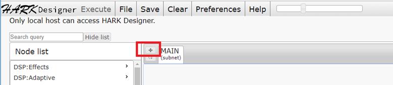
Figure 17. The '+' icon to add a new sheet - Name the new sheet LOOP0 and set its type to Iterator in the settings dialog box as shown in Figure 18a.
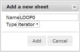
Figure 18a. "Add a new sheet" Dialog Box
Note that any name can be given to the new sheet and any newly created sheet's name will appear in the node list in the Dynamic category as shown in Figure 18b.
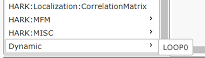
Figure 18b. "Dynamic" in the bottom of the Node List - Click on LOOP0 sheet and create a network as shown in Figure 19 below.
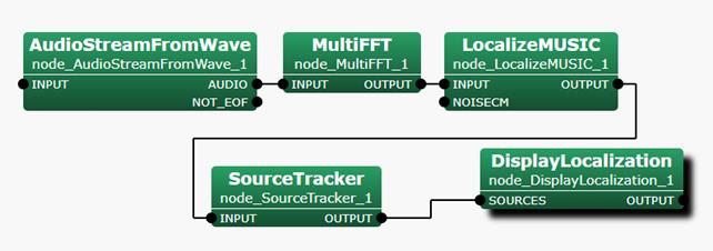
Figure 19. The sub network to be created in LOOP0
- The next steps are for creating the network in Figure 19.
-
Add the following five nodes in LOOP0 sheet; AudioStreamFromMic, MultiFFT, LocalizeMUSIC, SourceTracker and DisplayLocalization. These nodes are listed in the Node list or can also be found by typing the node name in the search field located above the node list. To add a node, click the node once it is displayed in the Node list. Figure 20 shows both the node list and the search field.
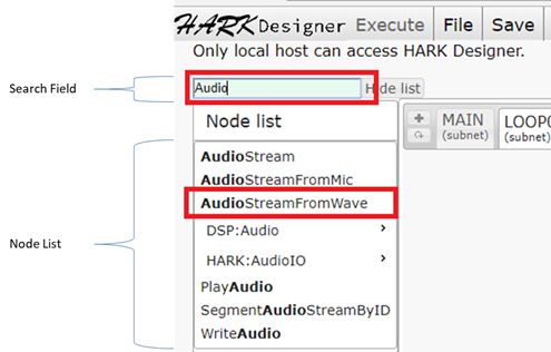
Figure 20. Search field and Node List
- After adding all five nodes, link all nodes, as shown in Figure 19.
Connect AudioStreamFromWave and MultiFFT (Figure 21) by dragging AudioStreamFromWave's output terminal named AUDIO to MultiFFT's INPUT terminal.. Repeat and apply this step to the other nodes in Figure 19.
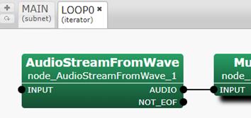
Figure 21. Connect AudioStreamFromWave and MultiFFT
- Right click on AudioStreamFromWave INPUT and click "Set as Input". See Figure 22 below.
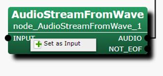
Figure 22. The setting option of INPUT
- After setting the INPUT, right click on AudioStreamFromWave's NOT_EOF output terminal, and click on "Set as Condition" as shown in Figure 23 below.
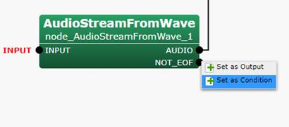
Figure 23. The setting options of NOT_EOF
- Double click on AudioStreamFromWave and set the following parameters as shown in Figure 24 below.
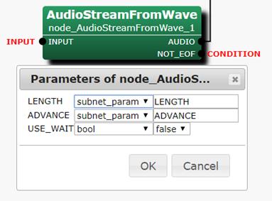
Figure 24. Parameters of node_AudioStreamFromWave dialog box
- Double click on MultiFFT and set the parameters as shown in Figure 25.
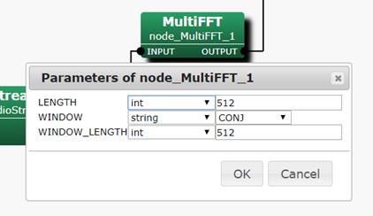
Figure 25. Parameters of node_MultiFFT dialog box
- Double click on LocalizeMUSIC and set the parameters as shown in Figure 26. TF_CHANNEL_SELECTION parameter should correspond to the number of channels of the microphone array that will be used in this network. A _MATRIX parameter should contain the name of the transfer function that was generated for the microphone array.
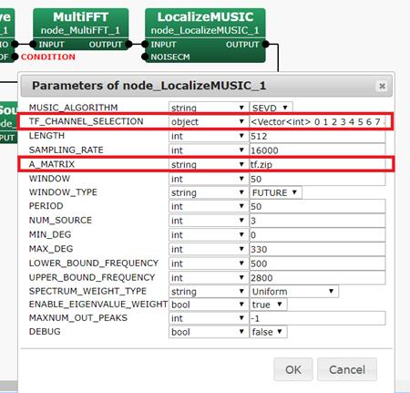
Figure 26. Parameters of node_LocalizeMUSIC dialog box
- Double click on SourceTracker. Set the parameters as shown in Figure 27.
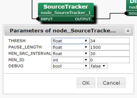
Figure 27. Parameters of node_SourceTracker dialog box
- Double click on DisplayLocalization and set the parameters as shown in Figure 28. PLOT_TYPE parameter can be set to any of the following: AZIMUTH, ELEVATION, X, Y AND Z. In this network, PLOT_TYPE will be set to AZIMUTH to show which angle the sound was recorded. Right click on DisplayLocalization OUTPUT and click "Set as Output" option.
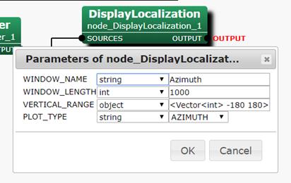
Figure 28. Parameters of node_DisplayLocalization dialog box
Sheet LOOP0 created in Step 3 is now ready to be used.
-
Add the following five nodes in LOOP0 sheet; AudioStreamFromMic, MultiFFT, LocalizeMUSIC, SourceTracker and DisplayLocalization. These nodes are listed in the Node list or can also be found by typing the node name in the search field located above the node list. To add a node, click the node once it is displayed in the Node list. Figure 20 shows both the node list and the search field.
- After setting the parameters of the five nodes added in LOOP0 (See Figure 19), click MAIN sheet of the HARK Designer as shown in Figure 29 below.
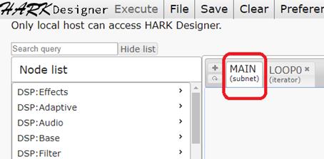
Figure 29. The MAIN sheet tab
- Enter LOOP0 in Search query field of the HARK Designer as shown in Figure 30, then click LOOP0 from the Node List to add LOOP0 Node in MAIN sheet.
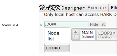
Figure 30. Highlight LOOP0 by typing the name in the search field
- Right click on LOOP0 OUTPUT and click "Set as Output" option as shown in Figure 31.
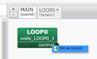
Figure 31. LOOP0 OUTPUT setting options
- Set the OUTPUT Name and use the default Name OUTPUT as shown in Figure 32 below then click OK.
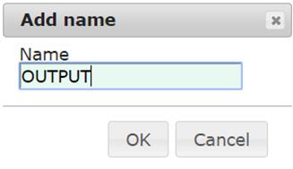
Figure 32. Add name Dialog box
- In the MAIN sheet, add Constant and InputStream nodes. Connect these nodes as shown in Figure 33.
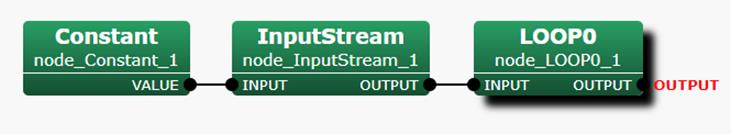
Figure 33. A completed network of MAIN sheet in HARK Designer
- Double click on Constant and set the parameters as shown in Figure 34. The value of Constant node's VALUE parameter should be that of the input recorded speech WAV file which will be used to evaluate the transfer function. Then click OK.
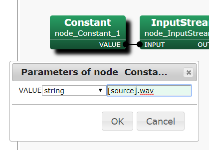
Figure 34. Parameter of node_Constant dialog box
- To be able to use the WAV file set in Constant node parameter in the previous step, you need to upload the WAV file to HARK Designer's path. To do this, click on 'File' and click 'Choose Files' as shown in Figure 35.
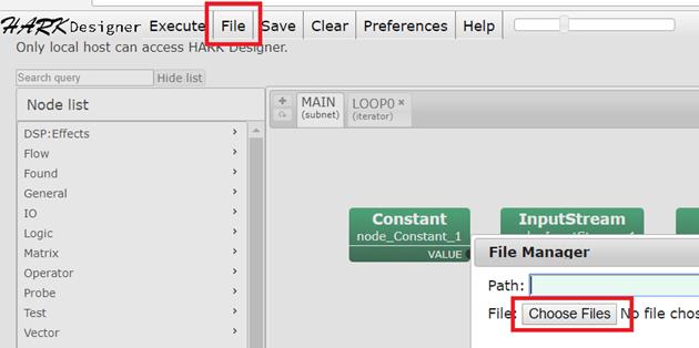
Figure 35. Uploading file in HARK Designer
- Locate the file to be uploaded and click OK in the "Network file name" dialog box shown in Figure 36.
- Click on the Save button at the top left part of HARK Designer, save Network file into preferred filename and click OK. See Figure 36 for the location of the Save button.
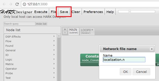
Figure 36. Save button
4.1.2. Executing a Network
To execute the network file created in the prior section, follow the steps below.
-
The first thing you will have to do before executing the network file is to load the network file itself. Let's begin by loading the network file we wish to execute. In our case, we will be using the network file created on Section 4.1.1. To do this, click on the 'File' button and locate the network file. Click on the 'Load' button as shown in Figure 37.
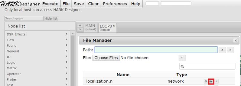
Figure 37. Loading a network file in HARK Designer
-
To execute a network file, click the Execute button at the top left part of HARK Designer as shown in Figure 38.
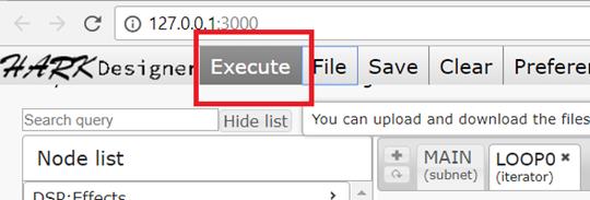
Figure 38. Execute button
-
Check the top right portion of the HARK Designer, and make sure there are no error messages. Figure 39 shows a successful execution of the network file.
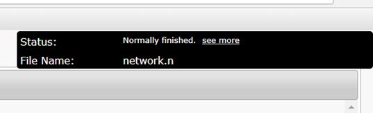
Figure 39. Successful execution of network file in HARK Designer
-
Figure 40 shows an unsuccessful execution of the network file. Click 'see more' to get more information about the failure.
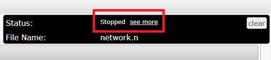
Figure 40. Error in executing a network file in HARK Designer
4.1.3. Evaluating the results
To see if we have successfully conducted Sound Source Localization using the transfer function we have created, follow the steps below.
- Execute the network file, please refer to Section 4.1.2 (Executing a Network file).
- When you execute the network file, a localization windows will appear as shown in Figure 41. Note: This Figure was taken on Ubuntu.
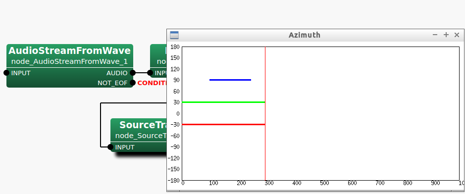
Figure 41. Visualization of the sound sources after Sound Source Localization
This window will display any sound sources located using the transfer function. Every time a new source is located, the source will be represented by a different color.
If every expected sound source was not located, please decrease the value of SoundTrackers's THRESH parameter and run the network file once more. If more sound sources were located than the ones expected, increase this value.
4.2. Evaluating Separation Transfer Functions
To evaluate the separation transfer functions, a network that separates a mixture of multiple sound sources needs be created. This network should have GHDSS. GHDSS requires a file containing separation transfer functions. The following sub section provides directions on how to create this network, how to execute the network, and how to confirm the result.
4.2.1. Creating a Network File
The following nodes are typically used in a network when sound source separation is needed:
- AudioStreamFromWave - reads speech waveform data from a WAV file. This node will read the recorded speech/simultaneous speech.
- MultiFFT - performs Fast Fourier Transforms (FFT) on multichannel speech waveform data.
- ConstantLocalization - continuously outputs constant sound source localization results.
- GHDSS - performs sound source separation based on the GHDSS (Geometric High-order Decorrelation-based Source Separation) algorithm. Transfer function of the microphone array is one of the files needed in this node.
- Synthesize - converts signals of frequency domain into waveforms of time domain.
- SaveWavePCM - saves speech waveform data in time domain as files.
The procedures to create a network to evaluate separation transfer functions are as follows:
- Launch HARK Designer.
- Windows: Double click the HARK Designer icon (Figure 42) on Desktop.
Figure 42. Hark Designer Icon
- Ubuntu: Open Terminal and run the following command:
$ hark_designer
Note: For HARK 2.4.0+ Firefox users, please use the following command:
$ hark_designer f
- Windows: Double click the HARK Designer icon (Figure 42) on Desktop.
- Once Hark Designer is launched, click the '+' icon next to the MAIN (subnet) sheet in the initial screen (Figure 43) to add a new sheet.
Figure 43. The '+' icon to add a new sheet - Name the new sheet MAIN_LOOP and set its type to Iterator in the "Add a new sheet" Dialog box (Figure 44). Note that any name can be given to the new sheet and any newly created sheet's name will appear in the node list in the Dynamic category..
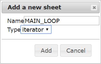
Figure 44. "Add a new sheet" Dialog Box
- Click on MAIN_LOOP sheet and create a network as shown in Figure 45.
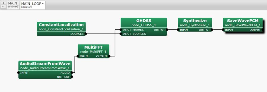
Figure 45. The sub network to be created in MAIN_LOOP
- The next steps are for creating the network in Figure 45.
-
Add the following six nodes in MAIN_LOOP sheet; AudioStreamFromWave, MultiFFT, ConstantLocalization, GHDSS, Synthesize and SaveWavePCM into MAIN_LOOP sheet. These nodes are listed in the Node list or can also be found by typing the node name in the search field located above the node list. To add a node, click the node once it is displayed in the Node list. Figure 46 shows both the node list and the search field.
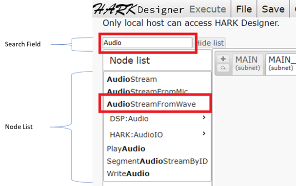
Figure 46. Search field and Node List
- After adding all five nodes, link all nodes, as shown in Figure 45.
Connect AudioStreamFromWave and MultiFFT (Figure 47) by dragging AudioStreamFromWave's output terminal named AUDIO to MultiFFT's INPUT terminal.
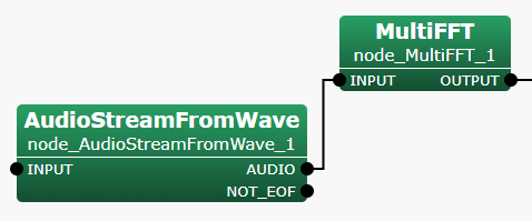
Figure 47. Connect AudioStreamFromWave and MultiFFT
- Now connect MultiFFT OUTPUT to GHDSS INPUT_FRAMES. See Figure 48 below on how to link these nodes.
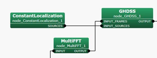
Figure 48. Connect MultiFFT and GHDSS
- Connect ConstantLocalization SOURCES to GHDSS INPUT_SOURCES as shown in Figure 49 below.
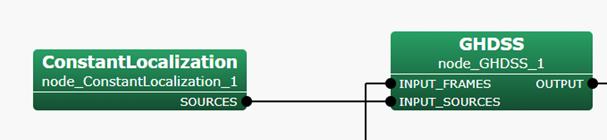
Figure 49. Connect ConstantLocalization and GHDSS
- Connect GHDSS OUTPUT to Synthesize INPUT as shown in Figure 50 below..
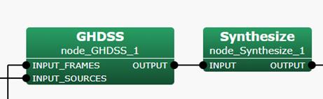
Figure 50. Connect GHDSS and Synthesize
- Connect Synthesize OUTPUT to SaveWavePCM INPUT as shown in Figure 51 below.
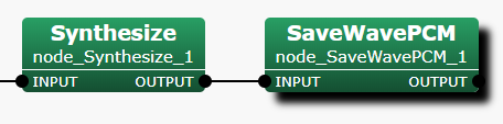
Figure 51. Connect Synthesize OUTPUT to SaveWavePCM INPUT
- Once all the nodes are connected as shown in Figure 45, set the parameters of each node.
Click AudioStreamFromWave, and right click on AudoStreamFromWave INPUT and click "Set as Output". See Figure 52 below.
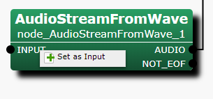
Figure 52. The setting option of INPUT
- After setting the INPUT, right click on AudioStreamFromWave NOT_EOF, and click on "Set as Condition" as shown in Figure 53 below.

Figure 53. The setting options of NOT_EOF
- Double click on AudioStreamFromWave and set the following parameters as shown in Figure 54.
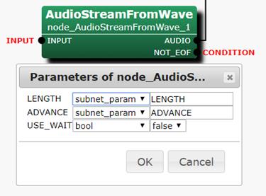
Figure 54. The values to set for AudioStreamFromWave parameters
- Double click on MultiFFT and set the parameters as shown in Figure 55.

Figure 55. The values to set for MultiFFT parameters - Double click on ConstantLocalization. On the ANGLES parameter as shown in Figure 56, set the values to the actual angles where the sound sources were recorded from. For instance, if the sound sources were recorded from angles 0°, 330° and 60°, the values should be set as followed <Vector<float> 0 330 60>.
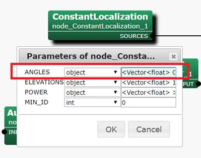
Figure 56. ANGLES parameter setting for ConstantLocalization - On the ConstantLocalization ELEVATIONS parameter shown in Figure 57, set the values to the elevation of each sound source, e.g. <Vector<float> 16.7 16.7 16.7>.
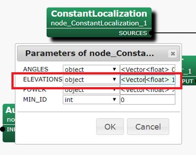
Figure 57. ELEVATIONS parameter setting for ConstantLocalization - On the ConstantLocalization POWER parameter shown in Figure 58, set the values to the power of each sound source. Leave it unset if you don't know the value.
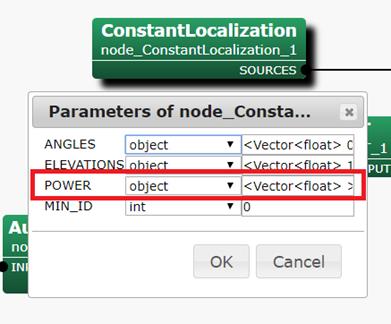
Figure 58. POWER Parameter setting for ConstantLocalization - After setting the parameters of ConstantLocalization, set parameters of GHDSS node. The GHDSS node performs sound source separation. Set the values of the parameters as shown in Figure 59. TF_CHANNEL_SELECTION parameter should correspond to the number of channels of the microphone array that will be used in this network. A _MATRIX parameter should contain the name of the transfer unction that was generated for the microphone array.
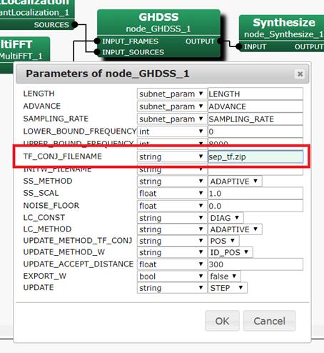
Figure 59. Transfer Function parameter setting for GHDSS - After setting the parameters of the GHDSS node, set the parameters of Synthesize node. Set the values of each parameter accordingly. You can refer to Figure 60 below for its values. OUTPUT_GAIN needs to be adjusted for instance, increase the value when the wave is too small and decrease the value when the wave is too large. Figure 45 enclose the OUTPUT_GAIN.
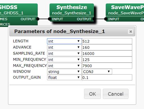
Figure 60. The values to set for Synthesize parameters - Right click on SaveWavePCM OUTPUT and click 'Set as Output' as shown in Figure 61. Set the OUTPUT name to its default OUTPUT name.
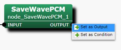
Figure 61. The setting options of OUTPUT - Set the OUTPUT Name and use the default Name OUTPUT as shown in Figure 62 below then click OK.

Figure 62. "Add name" Dialog box - Double click on SaveWavePCM. A dialog box will appear. We will be changing BASENAME and BITS parameters. BASENAME indicates the base name of the WAV file that will be saved using this node. Please change it to your preferred value. BITS parameter should match that of the MIC's output bit. For this value should set it to int24 as shown in Figure 63. Once done click OK.
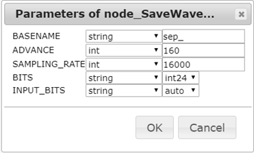
Figure 63. BASENAME parameter setting for SaveWavePCM
MAIN_LOOP sheet is now set and ready to be used.
-
Add the following six nodes in MAIN_LOOP sheet; AudioStreamFromWave, MultiFFT, ConstantLocalization, GHDSS, Synthesize and SaveWavePCM into MAIN_LOOP sheet. These nodes are listed in the Node list or can also be found by typing the node name in the search field located above the node list. To add a node, click the node once it is displayed in the Node list. Figure 46 shows both the node list and the search field.
- After setting the parameters of the five nodes added in MAIN_LOOP (See Figure 45), click the MAIN sheet of the HARK Designer as shown in Figure 64.
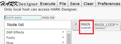
Figure 64. The MAIN sheet tab
- Enter MAIN_LOOP in Search query field of the HARK Designer as shown in Figure 65, then click MAIN_LOOP from the Node List to add MAIN_LOOP Node in MAIN sheet.
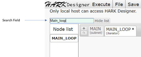
Figure 65. Adding MAIN_LOOP node to MAIN sheet in HARK Designer
- Right click on MAIN_LOOP OUTPUT and click "Set as Output" option as shown in Figure 66.
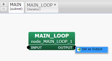
Figure 66. MAIN_LOOP OUTPUT setting options
- Set the OUTPUT Name and use the default Name OUTPUT as shown in Figure 67 below then click OK.
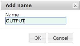
Figure 67. "Add name" Dialog box
- In the MAIN sheet, add Constant and InputStream nodes. Connect these nodes as shown in Figure 68.
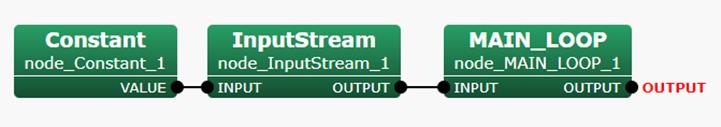
Figure 68. A completed sub network of MAIN sheet in HARK Designer
- Double click on Constant and set the parameters as shown in Figure 69. The value of the VALUE parameter should be the WAV file recorded with multiple simultaneous speakers.Then click OK.

Figure 69. "Parameter of node_Constant" Dialog box
- To be able to use the WAV file set in Constant node parameter in the previous step, you need to upload the WAV file to HARK Designer's path. To do this, click on 'File' and click 'Choose Files' as shown in Figure 70.
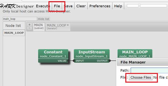
Figure 70. Uploading file in HARK Designer
- Locate the file to be uploaded and click OK.
- The network file is now ready to be saved.
- Click Save button at the top part of HARK Designer, save Network file into preferred filename and click OK. See Figure 71 for the location of the Save button.
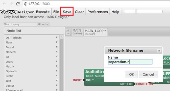
Figure 71. Save button
4.2.2. Executing a Network
To execute the network file created in Section 4.2.1, follow the steps below.
-
The first thing you will have to do before executing the network file is to load the network file itself. Let's begin by loading the network file we wish to execute. In our case, we will be using the network file created on Section 4.2.1. To do this, click on the ''File' button and locate the network file. Click on the 'Load' button as shown in Figure 72.
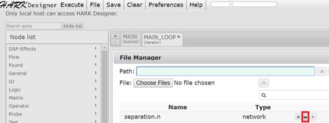
Figure 72. Load Button to load a network file
-
To execute a network file, click the execute button situated at the top part of HARK Designer as shown in Figure 73.
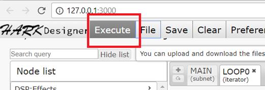
Figure 73. Execute button
-
Check the top right portion of the HARK Designer, and make sure there are no error messages. Figure 74 shows a successful execution of the network file.
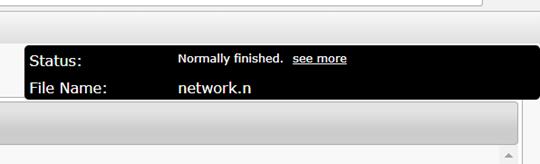
Figure 74. Successful execution of network file in HARK Designer
-
Figure 75 below shows an unsuccessful execution of the network file. Click 'see more' to get more information about the failure.
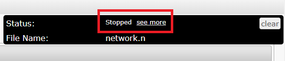
Figure 75. Error in executing a network file in HARK Designer
4.2.3. Evaluating the results
The results should generate 3 files because we have specified location information of 3 sound sources in ConstantLocalization in Section 4.2.1 as shown in Figure 76.
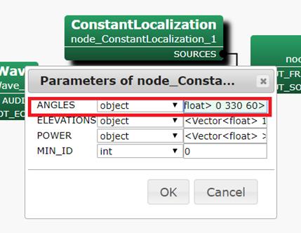
Figure 76. ConstantLocalization Parameters in Section 4.2.1
To check the results of the execution, follow the steps below:
- Run the Sound Source Separation network file. To run, please refer to Section 4.2.2 (Executing a Network file).
- After successfully executing the network, go to the HARK Designer folder. For Ubuntu users /usr/lib/hark-designe/userdata/network/ for Windows users, the default folder path is in C:/ProgramData/HARK/hark-designer/userdata/networks. Or click 'File' situated at the top of HARK Designer and take note of the value in 'Path' parameter as shown in Figure 77.
- Go to the HARK Designer path in Step 2 above. Note that in Section 4.2.1 Figure 63, the SaveWavePCM BASENAME parameter was set to sep_3src_.
- Check if sep_3src_0, sep_3src_1 and sep_3src_2 WAV files are generated. See Figure 78 for an illustration on how you should find the separated files.
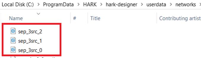
Figure 78. Output files generated after running the separation network
- Open the separated files in Audacity. Play each file, and check if all three sources were separated successfully.
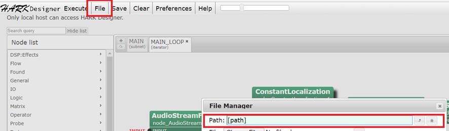
Figure 77. Path for the networks and other files in HARK Designer
---- End-----