SourceSeparation Node¶

Outline of the node¶

This node conducts blind sound source separation based on independent vector analysis.

Typical connection¶

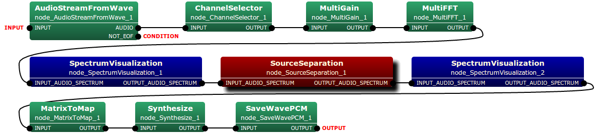
The type of both the input and output of SourceSeparation node is multi-channel (2-ch) audio spectrum. Typical connection of this node is depicted as follows:

Input-output and property of the node¶

Input¶

INPUT_AUDIO_SPECTRUM Matrix<complex<float> >: Windowed spectrum data. A row index is channel, and a column index is frequency.

Output¶

OUTPUT_AUDIO_SPECTRUM Matrix<complex<float> >: Windowed and speech-enhanced spectrum data . A row index is channel, and a column index is frequency.

Parameters¶

Parameters of this node are listed as follows:

Parameter name	Type	Default value	Unit	Description
FFT_LENGTH	int	512	sample	Analysis frame length.
ITERATION_METHOD	string	FastIVA		Iteration method.
MAX_ITERATION	int	700		Processing limitation: maximum number of iterations.
NUMBER_OF_SOURCE_TO_BE_SEPARATED	int	2		Number of sound sources to be separated.
SEPARATION_TIME_LENGTH	float	5.0	second	Separation window length.
ADVANCE	int	160	sample	The length in sample between a frame and a previous frame.
SAMPLING_RATE	int	16000	Hz	Sampling rate.

Details of the node¶

This module conducts recovery of the original sound signals from the combined sound signal by using independent vector analysis (IVA) [1] or Fast independent vector analysis (Fast-IVA) [2]. In the case of IVA, the objective function is Kullback-Leibler (KL) divergence:

\(C={\rm constant}- \sum^F_f {\rm log}\left|{\rm det} W_{mkf}\right| - \sum^M_m E\left[{\rm log}P \left( \hat{S}_1, \cdots ,\hat{S}_M \right)\right]\)

where \(\hat{S}_m (m = 1, \cdots, M)\) and \(W_{mkf}\) represent the input signal of m-th microphone and the separation matrix of IVA, respectively. The lerning algorithm of IVA is based on natural gradient-descent method:

\(W^{new}_{mkf}=W^{old}_{mkf} + \eta \sum^K_k \left( I_{mk} - E \left[ \frac{\hat{S}_{kf}}{\sqrt{\sum^F_f \left| \hat{S}_{kf} \right|^2}} \hat{S}_{kf}^{\ast} \right] \right) W^{old}_{mkf}\)

where \(\eta\) is learning rate (set at 0.1)

In the case of Fast-IVA, following modified objective function based KL divergence on is used:

\(C=-\sum^M_m E\left[{\rm log}P \left( \hat{S}_1, \cdots ,\hat{S}_M \right)\right] - \sum^M_m \beta\left[W^T_{mkf}W^{new}_{mkf}-1\right]\),

where \(\beta\) is Langrangian multiplier. The learning algorithm, on the other hand, is based on newton method with fixed point iteration:

\(W^{new}_{mkf}= E\left[\frac{1}{\sqrt{\sum^F_f \left|\hat{S}_{kf}\right|^2}} - \frac{\hat{S}^2_{kf}}{\left( \sqrt{\sum^F_f \left|\hat{S}_{kf}\right|^2}\right) ^3}\right] W^{old}_{mkf} -E\left[\frac{\hat{S}_{kf}}{\sqrt{\sum^F_f \left|\hat{S}_{kf}\right|^2}} X_{kf}\right]\)

References¶

[1]	Kim, H. T. Attias, S. Lee, and T. Lee, “Blind Source Separation Exploiting Higher-Order Frequency Dependencies,” IEEE Transactions on Audio, Speech, and Language Processing, vol. 15, no. 1, pp. 70–79, January 2007.

[2]	Lee, T. Kim, and T. Lee, “Fast fixed-point independent vector analysis algorithms for convolutive blind source separation” Signal Processing, vol. 87, no. 8, pp. 1859–1871, August 2007.